41 excel 2013 pie chart labels

Edit titles or data labels in a chart - support.microsoft.com On a chart, do one of the following: To edit the contents of a title, click the chart or axis title that you want to change. To edit the contents of a data label, click two times on the data label that you want to change. The first click selects the data labels for the whole data series, and the second click selects the individual data label. How to Add Axis Labels in Excel Charts - Step-by-Step (2022) - Spreadsheeto How to add axis titles 1. Left-click the Excel chart. 2. Click the plus button in the upper right corner of the chart. 3. Click Axis Titles to put a checkmark in the axis title checkbox. This will display axis titles. 4. Click the added axis title text box to write your axis label.

Excel charts: add title, customize chart axis, legend and data labels Click the Chart Elements button, and select the Data Labels option. For example, this is how we can add labels to one of the data series in our Excel chart: For specific chart types, such as pie chart, you can also choose the labels location. For this, click the arrow next to Data Labels, and choose the option you want.

Excel 2013 pie chart labels

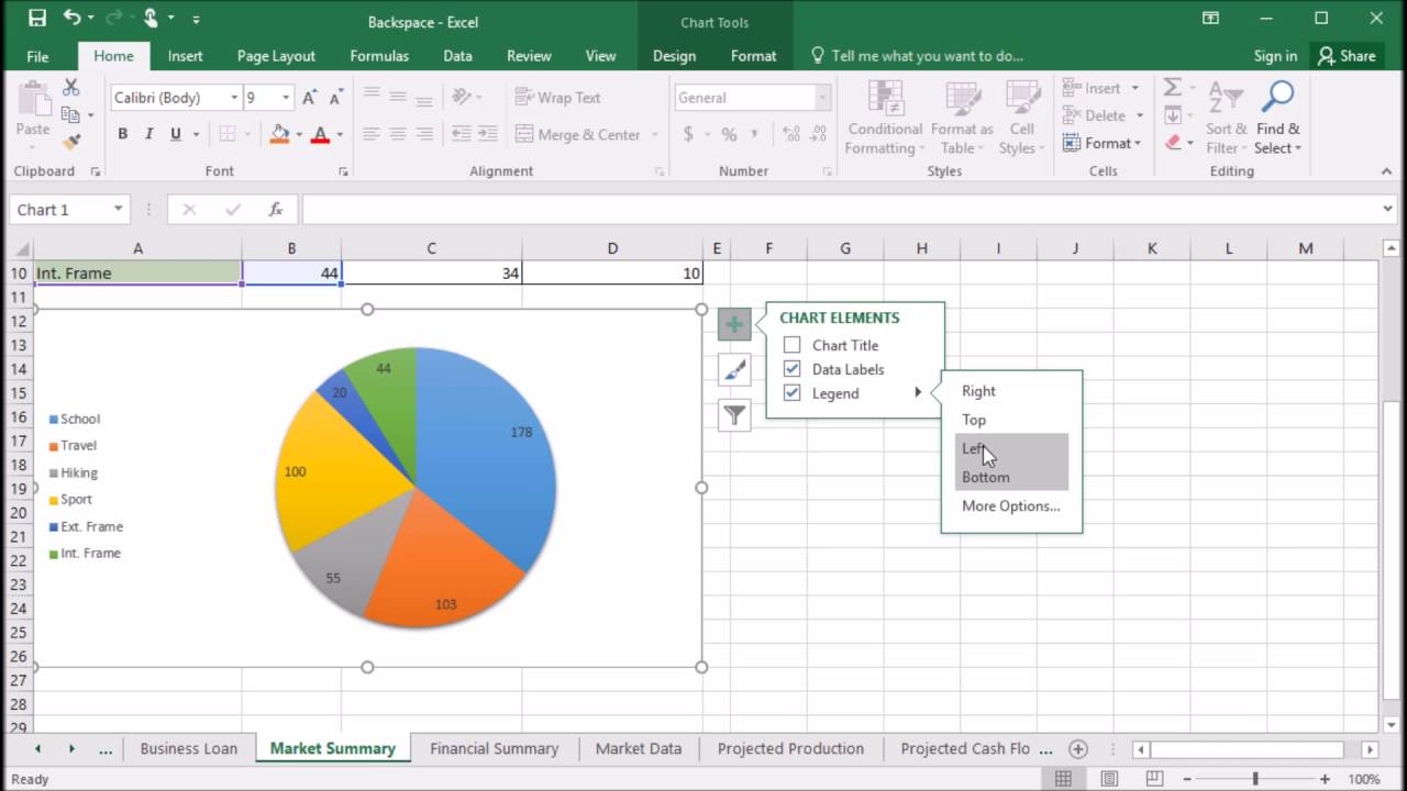
How to add or move data labels in Excel chart? - ExtendOffice In Excel 2013 or 2016. 1. Click the chart to show the Chart Elements button . 2. Then click the Chart Elements, and check Data Labels, then you can click the arrow to choose an option about the data labels in the sub menu. See screenshot: In Excel 2010 or 2007. 1. click on the chart to show the Layout tab in the Chart Tools group. See ... Adding rich data labels to charts in Excel 2013 | Microsoft 365 Blog You can do this by adjusting the zoom control on the bottom right corner of Excel's chrome. Then, select the value in the data label and hit the right-arrow key on your keyboard. The story behind the data in our example is that the temperature increased significantly on Wednesday and that appeared to help drive up business at the lemonade stand. Excel 2013 Chart label not displaying - excelforum.com The pie chart displays the wedge within the chart itself, but does not display the label. At the moment I have data labels with percentages. All other labels display, of which there are 7. I found a solution that fixes the problem each time it arises and that is to select Chart Tools/Format/Series 1 data labels and then Format Selection.

Excel 2013 pie chart labels. › doughnut-chart-in-excelDoughnut Chart in Excel | How to Create Doughnut Excel Chart? Doughnut Chart is a part of a Pie chart in excel Pie Chart In Excel Making a pie chart in excel can help you with the pictorial representation of your data and simplifies the analysis process. There are multiple kinds of pie chart options available on excel to serve the varying user needs. read more. A pie occupies the entire chart, but it will ... Excel 2013: Charts - GCFGlobal.org Select the cells you want to chart, including the column titles and row labels. These cells will be the source data for the chart. In our example, we'll select cells A1:F6. From the Insert tab, click the desired Chart command. In our example, we'll select Column. Choose the desired chart type from the drop-down menu. Microsoft Excel Tutorials: Add Data Labels to a Pie Chart - Home and Learn To add the numbers from our E column (the viewing figures), left click on the pie chart itself to select it: The chart is selected when you can see all those blue circles surrounding it. Now right click the chart. You should get the following menu: From the menu, select Add Data Labels. New data labels will then appear on your chart: How to add titles to Excel charts in a minute. - Ablebits In Excel 2013 the CHART TOOLS include 2 tabs: DESIGN and FORMAT. Click on the DESIGN tab. Open the drop-down menu named Add Chart Element in the Chart Layouts group. If you work in Excel 2010, go to the Labels group on the Layout tab. Choose 'Chart Title' and the position where you want your title to display.

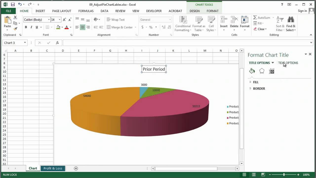
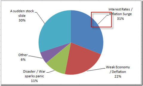
How to add axis label to chart in Excel? - ExtendOffice Click to select the chart that you want to insert axis label. 2. Then click the Charts Elements button located the upper-right corner of the chart. In the expanded menu, check Axis Titles option, see screenshot: 3. And both the horizontal and vertical axis text boxes have been added to the chart, then click each of the axis text boxes and enter ... Move and Align Chart Titles, Labels, Legends with the ... - Excel Campus Select the element in the chart you want to move (title, data labels, legend, plot area). On the add-in window press the "Move Selected Object with Arrow Keys" button. This is a toggle button and you want to press it down to turn on the arrow keys. Press any of the arrow keys on the keyboard to move the chart element. Display data point labels outside a pie chart in a paginated report ... To prevent overlapping labels displayed outside a pie chart. Create a pie chart with external labels. On the design surface, right-click outside the pie chart but inside the chart borders and select Chart Area Properties.The Chart AreaProperties dialog box appears. On the 3D Options tab, select Enable 3D. If you want the chart to have more room ... Format and customize Excel 2013 charts quickly with the new Formatting ... On the Ribbon, select the Chart Tools Format tab, then click Format Selection. The second way: On a chart, select an element. Right-click, then select Format where is the axis, series, legend, title, or area that was selected. Once open, the Formatting Task pane remains available until you close it.

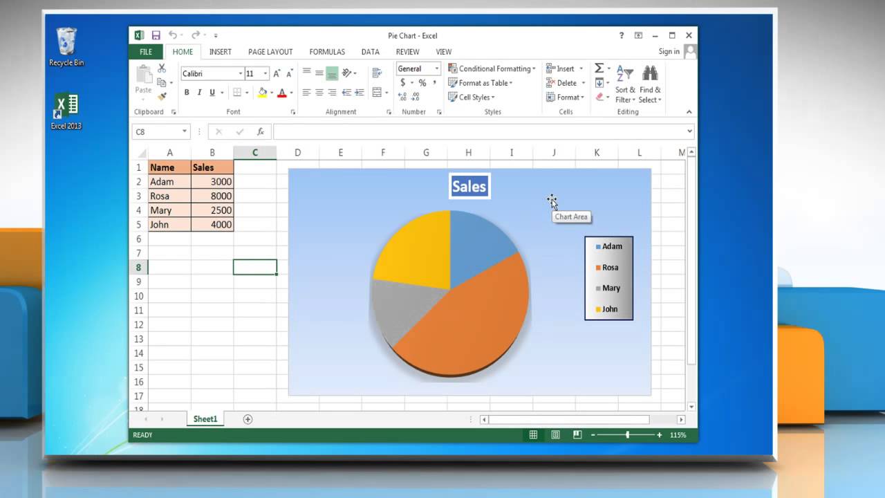
Excel 2013 Pie Chart Category Data Labels keep Disappearing GeneLandriau2 Created on April 19, 2016 Excel 2013 Pie Chart Category Data Labels keep Disappearing Hi All, I have a table in Excel 2013 with 2 slicers - Region and Product Hierarachy, with 5 values in each. I've built a couple pie charts that update when you click on the slicers, to show Market Share by Market Segment. support.microsoft.com › en-us › officeAdd a pie chart - support.microsoft.com To switch to one of these pie charts, click the chart, and then on the Chart Tools Design tab, click Change Chart Type. When the Change Chart Type gallery opens, pick the one you want. See Also. Select data for a chart in Excel. Create a chart in Excel. Add a chart to your document in Word. Add a chart to your PowerPoint presentation How to Create and Label a Pie Chart in Excel 2013 Open Microsoft Excel 2013 and click on the "Blank workbook" option. Tip Question Comment Step 2: Input the Data Create your spreadsheet by inputting the numbers and labels which are going to be used in the pie chart. In this example, I used the labels "Desserts", "Appertizers", "Entrees", "Beer", and "Wine". Tip Question Comment support.microsoft.com › en-us › officeChange the format of data labels in a chart To get there, after adding your data labels, select the data label to format, and then click Chart Elements > Data Labels > More Options. To go to the appropriate area, click one of the four icons ( Fill & Line , Effects , Size & Properties ( Layout & Properties in Outlook or Word), or Label Options ) shown here.

How to fix wrapped data labels in a pie chart | Sage Intelligence

Pie Chart - Remove Zero Value Labels - Excel Help Forum The formulas in the source table can be written in such a way as to mask the zero or error values, but they still show up in the chart. Solution (Tested in Excel 2010.): 1. Right click on one of the chart "data labels" and choose "Format Data Labels." 2. Choose "Number" from the vertical menu on the left. 3.

How to Adjust Pie Chart Labels in Excel : MS Excel Tips - YouTube

How to Label Axes in Excel: 6 Steps (with Pictures) - wikiHow Open your Excel document. Double-click an Excel document that contains a graph. If you haven't yet created the document, open Excel and click Blank workbook, then create your graph before continuing. 2. Select the graph. Click your graph to select it. 3. Click +. It's to the right of the top-right corner of the graph.

408 How format the pie chart legend in Excel 2016 - YouTube

How to Add Data Labels to your Excel Chart in Excel 2013 Data labels show the values next to the corresponding chart element, for instance a percentage next to a piece from a pie chart, or a total value next to a column in a column chart. You can choose...

Excel Dashboard Templates How-to Add Label Leader Lines to an Excel Pie Chart - Excel Dashboard ...

› ms-excel-pie-chartHow to Make a Pie Chart in Excel (Only Guide You Need) Jul 13, 2022 · Read More: How to Make Pie Chart in Excel with Subcategories (2 Quick Methods) Conclusion. Hope after reading this article you will not face any difficulties with the pie chart. This article covers all the necessary things regarding Excel Pie Chart. Stay tuned for more useful articles. Let us know what problems do you face with Excel Pie Chart.

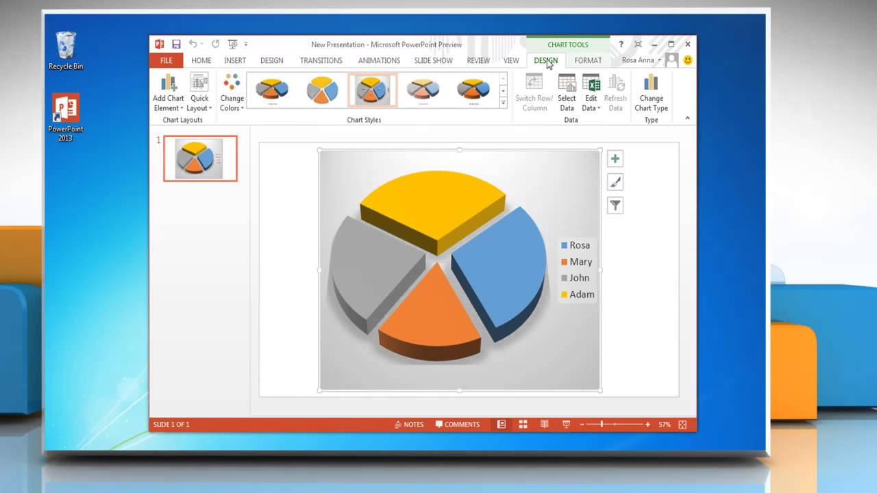
How to add data labels to a pie chart in Microsoft® PowerPoint 2013 presentation - YouTube

How to Insert Axis Labels In An Excel Chart | Excelchat We will again click on the chart to turn on the Chart Design tab. We will go to Chart Design and select Add Chart Element. Figure 6 - Insert axis labels in Excel. In the drop-down menu, we will click on Axis Titles, and subsequently, select Primary vertical. Figure 7 - Edit vertical axis labels in Excel. Now, we can enter the name we want ...

How to Create and Format a Pie Chart in Excel

Add or remove data labels in a chart - support.microsoft.com Click the data series or chart. To label one data point, after clicking the series, click that data point. In the upper right corner, next to the chart, click Add Chart Element > Data Labels. To change the location, click the arrow, and choose an option. If you want to show your data label inside a text bubble shape, click Data Callout.

Pie Chart – Excel Tutorials

How to Create and Format a Pie Chart in Excel - Lifewire To add data labels to a pie chart: Select the plot area of the pie chart. Right-click the chart. Select Add Data Labels . Select Add Data Labels. In this example, the sales for each cookie is added to the slices of the pie chart. Change Colors

How to Add an Axis Title to an Excel Chart | Techwalla.com

How to Use Cell Values for Excel Chart Labels - How-To Geek Select the chart, choose the "Chart Elements" option, click the "Data Labels" arrow, and then "More Options." Uncheck the "Value" box and check the "Value From Cells" box. Select cells C2:C6 to use for the data label range and then click the "OK" button. The values from these cells are now used for the chart data labels.

How to insert data labels in a Pie chart in Excel 2013 - YouTube

How to insert data labels to a Pie chart in Excel 2013 - YouTube This video will show you the simple steps to insert Data Labels in a pie chart in Microsoft® Excel 2013. Content in this video is provided on an "as is" basi...

How to Create and Format a Pie Chart in Excel

› charts › gauge-templateExcel Gauge Chart Template - Free Download - How to Create Step #7: Add the pointer data into the equation by creating the pie chart. Step #8: Realign the two charts. Step #9: Align the pie chart with the doughnut chart. Step #10: Hide all the slices of the pie chart except the pointer and remove the chart border. Step #11: Add the chart title and labels.

How to Create a Pie Chart in Microsoft Excel

Excel 2013 Chart Labels don't appear properly - Microsoft Community On PC A, an Excel Spreadsheet was created and from the data table, a pie chart was made which included data labels. See Attachment A. 2. PC A then emailed (using Outlook 2013) this excel spreadsheet, a Word 2013 doc containing a paste of this chart, and a powerpoint presentation 2013 containing the chart, to PC B and PC C 3.

Excel 3-D Pie charts - Microsoft Excel 2013

How to Add Data Tables to Charts in Excel 2013 - dummies To add a data table to your selected chart and position and format it, click the Chart Elements button next to the chart and then select the Data Table check box before you select one of the following options on its continuation menu: With Legend Keys to have Excel draw the table at the bottom of the chart, including the color keys used in the ...

32 How To Label A Pie Chart In Excel - Labels Information List

› 07 › 25How to create waterfall chart in Excel 2016, 2013, 2010 Jul 25, 2014 · A waterfall chart is also known as an Excel bridge chart since the floating columns make a so-called bridge connecting the endpoints. These charts are quite useful for analytical purposes. If you need to evaluate a company profit or product earnings, make an inventory or sales analysis or just show how the number of your Facebook friends ...

Legend help

How to modify Chart legends in Excel 2013 - Stack Overflow Right-click any column in the chart and select "Select Data" in the context menu. In the next dialog, select one of the series and click the Edit button. - teylyn. Apr 14, 2014 at 22:09. Thanks ... U may add the comment in main answer :)

Everything You Need to Know About Pie Chart in Excel

› excel-pie-chart-percentageHow to Show Percentage in Excel Pie Chart (3 Ways) Jul 03, 2022 · Display Percentage in Pie Chart by Using Format Data Labels. Another way of showing percentages in a pie chart is to use the Format Data Labels option. We can open the Format Data Labels window in the following two ways. 2.1 Using Chart Elements. To active the Format Data Labels window, follow the simple steps below. Steps:

Share :