38 excel pivot table labels
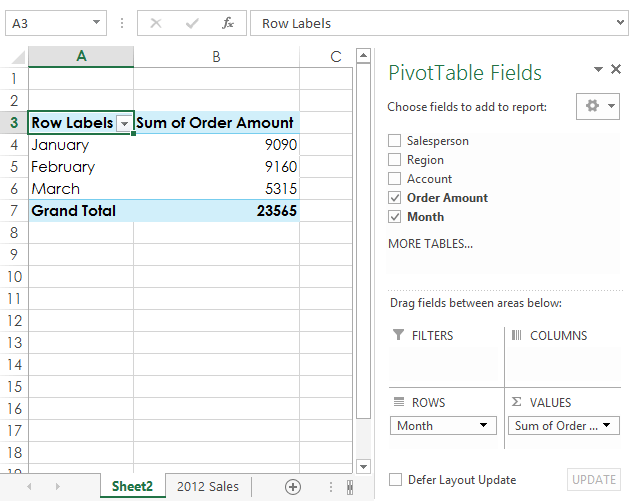
Excel tutorial: How to rename fields in a pivot table Either right-click on the field and choose Value field settings, or click Field Settings on the Options Tab of the PivotTable Tools ribbon. Here, you can see the original field name. In contrast to value fields, Row and Column label field names will be identical to the name in the field list. In fact, they are linked, as we'll see in a minute. How to Format Excel Pivot Table - Contextures Excel Tips Jul 09, 2021 · Change Pivot Table Labels. If you add fields to a pivot table's value area, the field labels show the summary function and the field name. For example, when you add a field named Quantity, it appears as "Sum of Quantity".
Changing Blank Row Labels - Excel Pivot Tables You can manually change the (blank) labels in the Row or Column Labels areas by typing over them in the pivot table. You can type any text to replace the (Blank) entry, but you can't clear the cell and leave it empty: Select one of the Row or Column Labels that contains the text (blank). Type N/A in the cell, and then press the Enter key.
Excel pivot table labels
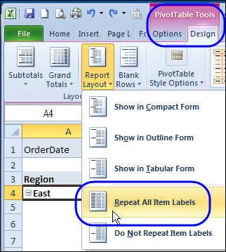
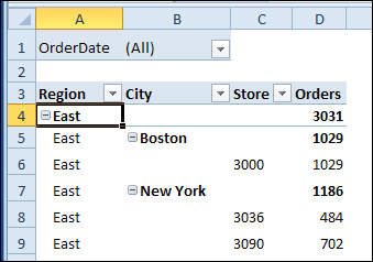
How to Move Excel Pivot Table Labels Quick Tricks To move a pivot table label to a different position in the list, you can use commands in the right-click menu: Right-click on the label that you want to move Click the Move command Click one of the Move subcommands, such as Move [item name] Up The existing labels shift down, and the moved label takes its new position. Type Over Another Label Pivot Table Row Labels In the Same Line - Beat Excel! After creating a pivot table in Excel, you will see the row labels are listed in only one column. But, if you need to put the row labels on the same line to view the data more intuitively and clearly as following screenshots shown. How could you set the pivot table layout to your need in Excel? Pivot table row labels in separate columns • AuditExcel.co.za Our preference is rather that the pivot tables are shown in tabular form (all columns separated and next to each other). You can do this by changing the report format. So when you click in the Pivot Table and click on the DESIGN tab one of the options is the Report Layout. Click on this and change it to Tabular form.
Excel pivot table labels. Pivot Table "Row Labels" Header Frustration - Microsoft ... Hi Everyone please help I can't change my headers from Row Labels in a Pivot Table. Using Excel 365 How To Flip A Pivot Table In Excel - Enjoytechlife Process of Flipping Pivot Table in Excel. In order to flip the pivot table, you must first launch the PivotTable & PivotChart Wizard context menu and then generate a fresh pivot table in Microsoft Excel. To enter the PivotTable & PivotChart Wizard box, tap the Alt+D+P keyboard shortcuts together. Pick Multiple consolidations ranges from the ... Excel filtering pivot table filter/slicer across column label Excel filtering pivot table filter/slicer across column label. Hello. I have a table with the year as the column headings/labels (2009-2021) and a couple other columns with additional information that aren't a year. The rows represent the specific data for each year. I have made a pivot table and slicers for the columns with the other date but ... Turn Repeating Item Labels On and Off - Excel Pivot Tables Select a cell in the pivot field that you want to change On the PIVOT POWER Ribbon tab, in the Pivot Items group, click Show/Hide Items Click Repeat Item Labels - On or Repeat Item Labels - Off To set the Default Setting: On the PIVOT POWER Ribbon tab, in the Formatting group, click Set Defaults
EXCEL: SETTING PIVOT TABLE DEFAULTS - Strategic Finance Apr 01, 2017 · Open the workbook that contains the pivot table. Select one cell in the pivot table. Go to File, Options, Advanced, Data, and click the button for Edit Default Layout. Use the Layout Import feature by entering a single cell from the pivot table in Layout Import and clicking the Import button. All of the settings from the pivot table will become ... Microsoft Excel - showing field names as headings rather ... In Microsoft Excel 2007 and 2010, by default if you create a pivot table, instead of showing the field names, it will say row labels and column labels. Show in Outline Form or Show in Tabular form. The relevant labels will To see the field names instead, click on the Pivot Table Tools Design tab,… How to rename group or row labels in Excel PivotTable? 1. Click at the PivotTable, then click Analyze tab and go to the Active Field textbox. 2. Now in the Active Field textbox, the active field name is displayed, you can change it in the textbox. You can change other Row Labels name by clicking the relative fields in the PivotTable, then rename it in the Active Field textbox. How to Customize Your Excel Pivot Chart Data Labels - dummies The Data Labels command on the Design tab's Add Chart Element menu in Excel allows you to label data markers with values from your pivot table. When you click the command button, Excel displays a menu with commands corresponding to locations for the data labels: None, Center, Left, Right, Above, and Below.
Remove PivotTable Duplicate Row Labels [SOLVED] Re: Remove PivotTable Duplicate Row Labels. Sometimes when the cells are stored in different formats within the same column in the raw data, they get duplicated. Also, if there is space/s at the beginning or at the end of these fields, when you filter them out they look the same, however, when you plot a Pivot Table, they appear as separate ... Repeat All Item Labels In An Excel Pivot Table - MyExcelOnline You can then select to Repeat All Item Labels which will fill in any gaps and allow you to take the data of the Pivot Table to a new location for further analysis. STEP 1: Click in the Pivot Table and choose PivotTable Tools > Options (Excel 2010) or Design (Excel 2013 & 2016) > Report Layouts > Show in Outline/Tabular Form How to reset a custom pivot table row label Thanks - I'm trying to edit the pivot table manually. I tried reformatting as you described to no avail. I'm trying to figure out how get rid of all cutomized labels. See example below using Excel 2007. Table starts like this: But then gets accidently edited to show like the one below. How to add column labels in pivot table [SOLVED] Steps:-. Click any date in the Column Lables. Click Pivot table options tab on the Ribbon. In the Options Table, Click Group Field option. Click Months then click Ok. Thats it. check the attached file:-. Attached Files. PIVOT.xlsx (30.3 KB, 6 views) Download.
Excel Advanced Dashboard
How to Use Label Filters for Text in the Pivot Table? - MS ... When you select the field name, the selected field name will be inserted into the pivot table. Pro Tip. Row Labels are used to apply a filter to rows that have to be shown in the pivot table. By default, it will show you the sum or count values in the pivot table.
MS Excel 2013: Display the fields in the Values Section in a single column in a pivot table
Use column labels from an Excel table as the rows in a ... Close the dialog and keep the changes. Excel should place the unpivoted data into a new worksheet, looking something like this: Now the final step is to create a pivot table using this unpivoted data. Here is a screenshot of my pivot table setup: Note that Attribute (e.g. Malaria, Tuberculosis) is placed above the Year. This lets us open or ...

How to Sort Pivot Table Row Labels, Column Field Labels and Data Values with Excel VBA Macro ...
How to unbold Pivot Table row labels - MrExcel Message Board Under the binocular tab, called FIND AND SELECT, select SELECT OBJECTS. This should place a thin blue line around that and all other subtotals at the same level. Make the changes you want (such as unbolding). P pschommer New Member Joined Nov 18, 2006 Messages 10 Dec 10, 2010 #3 After turning on 'Select Objects', the Font options are grayed out.

Use the Field List to arrange fields in a PivotTable - Excel
Repeat item labels in a PivotTable Right-click the row or column label you want to repeat, and click Field Settings. Click the Layout & Print tab, and check the Repeat item labels box. Make sure Show item labels in tabular form is selected. Notes: When you edit any of the repeated labels, the changes you make are applied to all other cells with the same label.

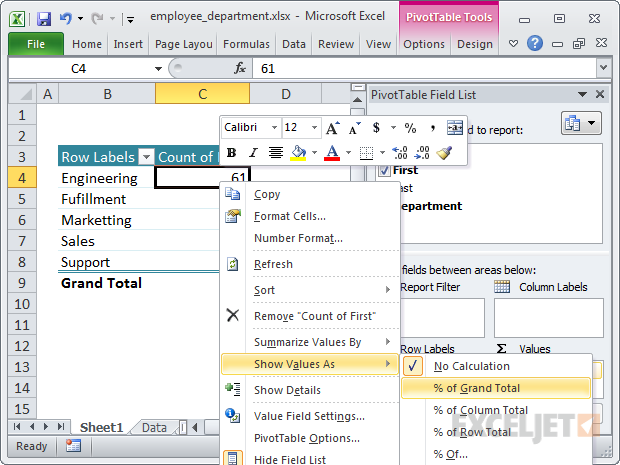
How to Show the Percentage of Row Total in the Pivot Table - MS Excel | Excel In Excel
How to make row labels on same line in pivot table? Make row labels on same line with PivotTable Options You can also go to the PivotTable Options dialog box to set an option to finish this operation. 1. Click any one cell in the pivot table, and right click to choose PivotTable Options, see screenshot: 2.
Excel Pivot Table group by month label format - Microsoft Community
Design the layout and format of a PivotTable In the PivotTable Options dialog box, click the Layout & Format tab, and then under Layout, select or clear the Merge and center cells with labels check box. Note: You cannot use the Merge Cells check box under the Alignment tab in a PivotTable. Change the display of blank cells, blank lines, and errors
MS Excel 2011 for Mac: Display the fields in the Values Section in multiple columns in a pivot table
Pivot table row labels side by side - Excel Tutorials You can copy the following table and paste it into your worksheet as Match Destination Formatting. Now, let's create a pivot table ( Insert >> Tables >> Pivot Table) and check all the values in Pivot Table Fields. Fields should look like this. Right-click inside a pivot table and choose PivotTable Options…. Check data as shown on the image below.

How to Sort Pivot Table Row Labels, Column Field Labels and Data Values with Excel VBA Macro ...
How to Customize Your Excel Pivot Chart and Axis Titles ... The Chart Title and Axis Titles commands, which appear when you click the Design tab's Add Chart Elements command button in Excel, let you add a title to your chart titles to the vertical, horizontal, and depth axes of your chart. In Excel 2007 and Excel 2010, you use the Chart Title and Axis Titles commands on the Layout tab to add chart and axis titles. After you choose the Chart ...

Excel Pivot Table Report - Sort Data in Row & Column Labels & in Values Area, use Custom Lists
Change Blank Labels in a Pivot Table - Contextures Blog In a pivot table, you might have a few row labels or column labels that contain the text "(blank)". This happens if data is missing in the source data. For example, in the source data, there might be a few sales orders that don't have a Store number entered.

Solved: Report a Table like Excel Pivot Table - Microsoft Power BI Community
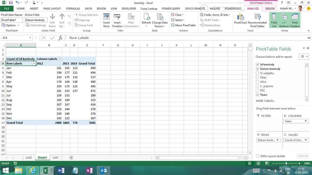
Microsoft Excel - showing field names as headings rather ... In earlier versions, by default if you create a pivot table, instead of showing the field names, it will say row labels and column labels. To see the field names instead, click on the Pivot Table Tools Design tab, then in the Layout group, click the Report Layout dropdown and select either Show in Outline Form or Show in Tabular form.

Accelerate Your Analysis with Pivot Table | Simplified Excel
Change the pivot table "Row Labels" text | MrExcel Message ... Feb 4, 2021. #3. mart37 said: Click on the cell and typ the text. Click to expand... Thanks mart37. So simple! I was looking for a way to change it on the ribbons & settings. Typical Excel - things you think are difficult are easy, and things that should be easy are difficult!
Pivot Table Excel 2013 | Decorations I Can Make
How to Group Numbers in Pivot Table in Excel Sometimes, numbers are stored as text in Excel. In such case, you need to convert these text to numbers before grouping it in Pivot Table. You May Also Like the Following Pivot Table Tutorials: How to Group Dates in Pivot Table in Excel. How to Create a Pivot Table in Excel. Preparing Source Data For Pivot Table. How to Refresh Pivot Table in ...
Repeat Pivot Table Labels in Excel 2010 - Excel Pivot TablesExcel Pivot Tables
Automatic Row And Column Pivot Table Labels Apr 18, 2018 — Learn this Excel Pivot Table tip which will quickly give you the correct row and column labels with a couple of clicks.
36 Which Is A Valid Column Label - Labels 2021
Hide Excel Pivot Table Buttons and Labels Jan 29, 2020 · The field labels – Year, Region, and Cat – are hidden, and they weren’t really needed. The pivot table summary is easy to understand without those labels. NOTE: You can still sort and filter the pivot fields, if you right-click on a cell, and use the commands in the pop-up menu. More Pivot Table Tips. Go to my Contextures website for more ...

EXCEL: SETTING PIVOT TABLE DEFAULTS - Strategic Finance
Excel 2016 Pivot table Row and Column Labels - Microsoft ... In Excel 2016 I've found when I create a pivot table it unhelpfully shows 'Row Labels' and 'Column Labels' instead of my field names, although in the top left cell it says 'Count of' and then inserts the correct field name. Years ago when I last used Excel it automatically put the field names in all three heading cells.

Tutorial 2: Pivot Tables in Microsoft Excel: Tutorial 2: Pivot Tables in Microsoft Excel
get a row label from pivot table - Microsoft Tech Community Alternatively you may work with cube assuming you are at least on Excel 2010, as I remember it's the first which supports data model. Create PivotTable and after that convert it to cube formulas. Now you may take these formulas and convert it to form you need, for example. =CUBEVALUE( "ThisWorkbookDataModel", CUBEMEMBER("ThisWorkbookDataModel ...
Repeat Pivot Table Labels in Excel 2010 – Excel Pivot Tables
The Pivot table tools ribbon in Excel Here are all the observational notes using the formula in Excel Notes : Create new pivot table columns using pivot table fields option under the analyze tab of pivot table ribbon in excel. Sort the data after filtering which makes it easier to read. You can create a pivot table on the same sheet as data or in a different sheet of the same workbook.

Excel Pivot Table Report - Sort Data in Row & Column Labels & in Values Area, use Custom Lists
How to Use Excel Pivot Table Label Filters In an Excel pivot table, you might want to hide one or more of the items in a Row field or Column field. To do that, you could click the drop down arrow for the Row or Column Labels, then remove the check mark for items you want to remove. For example, to hide the data for 7-Feb-10, you'd click on the check mark to remove it.
Post a Comment for "38 excel pivot table labels"